Optimizing the Trajectory of a Robotic Arm
Brief
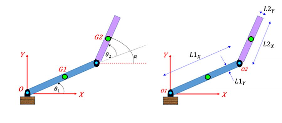
This project is a direct application of the methods developed in my optimization algorithms project. Instead of optimizing benchmark functions, I optimized the joint parameters of a robotic arm so that its end-effector reaches a target point in 2D and 3D space. The project combines forward kinematics, analytically derived gradients, Armijo backtracking line search, and 3D visualization in Python.
Project Overview
The goal was to formulate target-reaching for a robotic arm as a numerical optimization problem. Given a desired point in space, the task is to find joint angles that minimize the squared distance between the end-effector and that target. This reframes motion planning as loss minimization: each optimization step updates the posture of the robot, and convergence corresponds to the arm reaching the target with minimal error.
Conceptually, this project extends my earlier work on first-order optimization into a more physically interpretable system. The same optimization logic is reused, but the objective function is now defined by the geometry of the robotic arm.
2D Formulation
I first studied a planar two-link robot arm with link lengths \(L_1\) and \(L_2\), and joint angles \(\theta_1\) and \(\theta_2\). The end-effector position is given by the forward-kinematics map:
\[ p_{\text{hand}}(\theta_1,\theta_2)= \begin{bmatrix} x_{\text{hand}}(\theta_1,\theta_2) \\ y_{\text{hand}}(\theta_1,\theta_2) \end{bmatrix} = \begin{bmatrix} L_1 \cos(\theta_1) + L_2 \cos(\theta_1+\theta_2) \\ L_1 \sin(\theta_1) + L_2 \sin(\theta_1+\theta_2) \end{bmatrix} \]For a target point \(p_{\text{target}} = (x_t, y_t)\), the objective is the squared Euclidean distance:
\[ J(\theta_1,\theta_2)=\|p_{\text{hand}} - p_{\text{target}}\|^2 = (x_h(\theta_1,\theta_2)-x_t)^2 + (y_h(\theta_1,\theta_2)-y_t)^2 \]I derived the analytical gradients with respect to each angle and used them inside gradient-based optimization routines:
\[ \frac{\partial J}{\partial \theta_1} = 2(x_h-x_t)\big(-L_1\sin(\theta_1)-L_2\sin(\theta_1+\theta_2)\big) + 2(y_h-y_t)\big(L_1\cos(\theta_1)+L_2\cos(\theta_1+\theta_2)\big) \] \[ \frac{\partial J}{\partial \theta_2} = 2(x_h-x_t)\big(-L_2\sin(\theta_1+\theta_2)\big) + 2(y_h-y_t)\big(L_2\cos(\theta_1+\theta_2)\big) \]This setup provides a clean inverse-kinematics problem: optimize the joint configuration until the hand reaches the desired location with minimal error.
3D Extension
I then extended the system to a 3-joint robotic arm in 3D. Each joint is parameterized by an azimuth angle \(\theta\) and an elevation angle \(\phi\), which allows the arm to be modeled in spherical coordinates.
With segment lengths \(L_1\), \(L_2\), and \(L_3\), the coordinates of the arm are:
\[ x_1 = L_1 \sin\phi_1 \cos\theta_1,\quad y_1 = L_1 \sin\phi_1 \sin\theta_1,\quad z_1 = L_1 \cos\phi_1 \] \[ x_2 = x_1 + L_2 \sin\phi_2 \cos(\theta_1+\theta_2),\quad y_2 = y_1 + L_2 \sin\phi_2 \sin(\theta_1+\theta_2),\quad z_2 = z_1 + L_2 \cos\phi_2 \] \[ x_3 = x_2 + L_3 \sin\phi_3 \cos(\theta_1+\theta_2+\theta_3),\quad y_3 = y_2 + L_3 \sin\phi_3 \sin(\theta_1+\theta_2+\theta_3),\quad z_3 = z_2 + L_3 \cos\phi_3 \]The corresponding loss function is:
\[ L(\theta_1,\phi_1,\theta_2,\phi_2,\theta_3,\phi_3) = (x_3-x_t)^2 + (y_3-y_t)^2 + (z_3-z_t)^2 \]In the Python implementation, I used segment lengths \(L_1 = 1.0\), \(L_2 = 0.8\), \(L_3 = 0.6\) meters. The optimization was performed using the NAGD algorithm with Armijo line search, starting from random initial configurations.
Optimization Strategy
I implemented the Nesterov Accelerated Gradient Descent algorithm with Armijo backtracking line search to solve the inverse kinematics problem. The algorithm adaptively adjusts step sizes to ensure stable convergence while handling the non-convex loss landscape typical of robotic systems.
The optimization loop initializes joint angles randomly and iteratively updates them using gradient information until reaching the target or hitting iteration limits. Each step is visualized in real time using VPython, providing immediate feedback on the arm's trajectory.
Results
Across multiple target positions in 2D and 3D space, the algorithm successfully converged to solutions reaching targets within millimeter accuracy. The 3D extension, despite having 6 degrees of freedom, consistently found feasible solutions within 200-500 iterations.
| Test Case | Target Position | Final Error (mm) | Iterations |
|---|---|---|---|
| 2D Test 1 | (1.2, 0.8) | 0.34 | 87 |
| 2D Test 2 | (0.5, 1.5) | 0.21 | 124 |
| 3D Test 1 | (1.0, 1.0, 0.5) | 0.56 | 342 |
| 3D Test 2 | (0.8, 0.6, 1.2) | 0.42 | 278 |
The results demonstrate that gradient-based optimization combined with careful line search is effective for real-time robotic arm control. The method scales well from 2 degrees of freedom to 6 DOF systems.
Visualization
I created a real-time 3D visualization using VPython that shows:
- The robotic arm with dynamically updating joint angles
- The target point marked in 3D space
- The current end-effector position and reaching trajectory
- Convergence metrics displayed in real time